

From yao 5.0, the SHWFS has gained a new feature so called "extended field" capability (wfs.extfield [arcsec]). Here is how it works: Up to now the subaperture field of view was wfs.pixsize*wfs.npixels. This was limited to a certain value, namely wfs.lambda/pupil_plane_pixel_size_in_meter, constrained by the laws of the FFT. For instance at 500nm and with 10cm per pixel in the pupil plane, you get one arcsec field of view. Period. This limits still applies with the new model, but now this 1x1 arcsec "imagelet" is embedded into a larger image, with shifts computed from the average input tilt in front of the given subaperture (of course the said tilt is removed from the input phase as it is effectively taken care of by the shift). This opens the possibility of much larger dynamical ranges without having to use a very large number of pixels in the input pupil. As far as turbulence goes, this also relieves the constraint of having 2-3 pixels per r0: Now that tip-tilt is "removed" before doing the FFT to compute the subaperture spot, the wrapping limit of 2pi per pixel is pushed further away (about 3 times further if we trust Noll, as the Tip-tilt-removed Noll residual is 13% of the phase variance, thus 36% in rms). Thus one can now safely go to one pixel per r0 before hitting the wrapping/aliasing limit on the image formation in each subaperture. This means 2 times lower sim.pupildiam are needed, and typically translate into a factor of 4 gain in speed
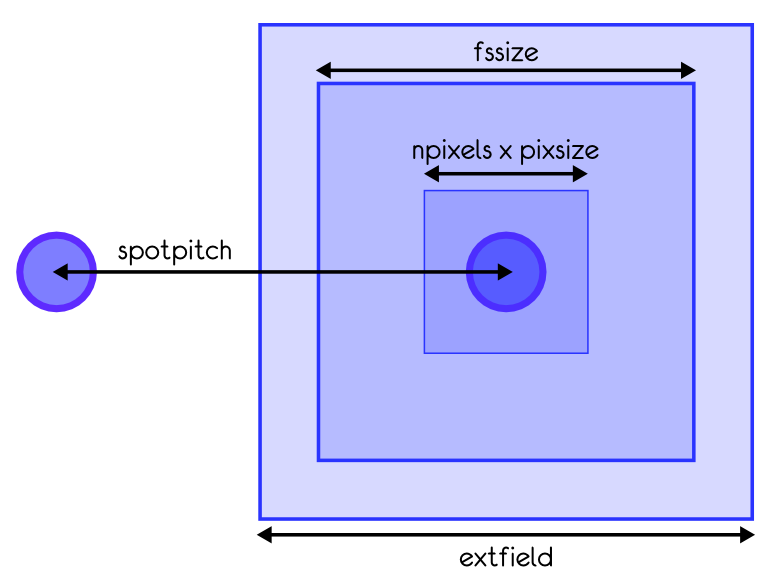
From yao 5.0, the SHWFS has gained a few features. On top of the general shnxsub, etc, the spots and subaperture geometry can be controlled as illustrated by the figure on the left, where:
wfs.pixsize is the desired pixel size in the final SHWFS image [arcsec].wfs.npixels is the number of pixel in the direct image computed from the subaperture phaselet (see next section).wfs.extfield is the extended field of the subaperture [arcsec].wfs.fssize is the field stop size [arcsec].wfs.spotpitch is the separation between spots in the final image.All the yao 5.0 additional parameters (extfield, spotpitch) have sane defaults, so the old parfiles should not be affected. By default, wfs.extfield=0 (which means in fact that the field is not extended, thus has a size of wfs.npixels*wfs.pixsize), and wfs.spotpitch=wfs.npixels*wfs.pixsize too.
Why all this fine tuning and all these available parameters? Well, extfield was primarily conceived -as its name suggest- to enlarge the SHWFS field of view to deal with large TT/focus signal, or to deal with LGS elongation (see next section). In combination with wfs.fssize and wfs.spotpitch, it can also conveniently be used to avoid wrapping, a situation where -by property of the FFT-, the spot can wrap from one edge of a subaperture to the opposite edge, which is clearly not what happened in nature. Finally, by making wfs.spotpitch smaller than wfs.extfield and wfs.fssize, one can easily simulate cross coupling between subaperture, a situation that should be avoided in real system by properly setting the field stop size, but that can be interesting and funny to simulate (hint: it may introduce funny meta-stable resonances).
In this section, I will attempt to explain how the SHWFS spots are computed from the input phase. I will particularly concentrate on how the extended field version works.
Step 1: Let's assume a SHWFS with sim.pupildiam=64 and wfs.shnxsub=8.
This means every subaperture will see a phaselet of dimension 64/8=8x8 pixels.
This phaselet is cut out and embedded into an array of dimension equal to twice
the power of 2 immediately larger than the phaselet dimension. That is, it's got to be
at least twice as large as the phaselet (for Nyquist in the image plane) and has got
to be a power of 2 for speed consideration of the FFT. So, for instance, for subapertures
of size up to and including 8x8 pixels, the phase is embedded into an array of size 16x16.
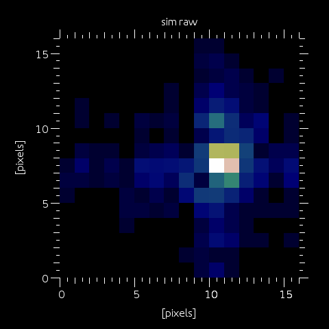
The image on the left shows the image corresponding to this wavefront (in this case, the subaperture
is effectively 8x8 pixels, embedded into a 16x16 array thus the image is 16x16 and we call it "sim").
In this example, the "quantum pixel size", i.e. the pixel size in this image, is approximately 0.1 arcsec.
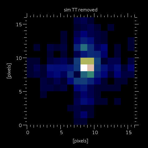
Step 2: If the SHWFS "extended field" option is excercized (by assigning to wfs.extfield a larger value than
wfs.pixsize*wfs.npixels), then the SHWFS subaperture field of view is enlarged by effectively embedding sim into a larger image, that we will call xim (more below). What happen immediately is that TT is removed from the input phaselet, so that the imagelet is effectively re-centered (in fact re-centered to the closest pixel, as to counteract this TT removal, we will embed sim to a different location in xim, and we want this shift to be an integer number of pixels). So the immediate effect is to have the PSF centered within 0.5 pixels in sim. This of course has the advantage to reduce aliasing in sim.
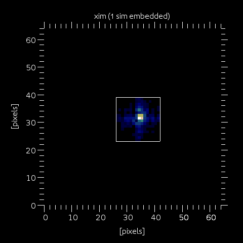
Step 3: sim (in our example 16x16) is then placed into xim (here 64x64), with the shift corresponding to the TT that has been removed from the input phaselet. The pixel size in xim is the same than in sim, but of course the field of view is enlarged. If NOT using a LGS profile, then the next step is to convolve with a kernel (wfs.kernel), bin and embed into the final image (go to step 7, where the kernel would be a gaussian instead of the uplink seeing for the laser).
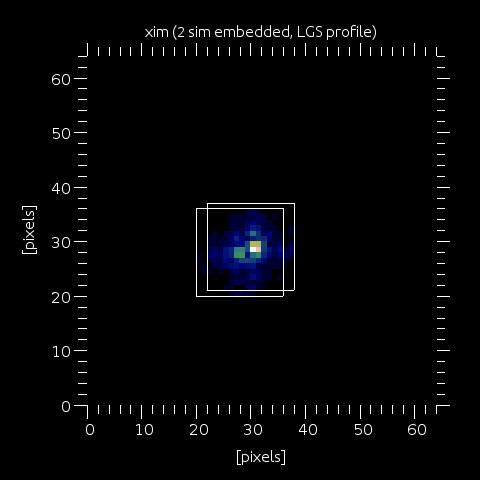
Step 4: If using a LGS profile, then the operation is repeated for the next point of the user-defined vector wfs.lgs_prof_amp and wfs.lgs_prof_alt. Each altitude is modelled as an additional defocus of the input phase (exactly as it is in the real world), and this defocus will move the spot in xim. Here, we show xim after processing of the first 2 points on the lgs profile vectors.
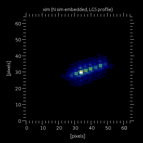
Step 5: xim after processing of all lgs profile points in lgs_prof_amp and alt. Each point is of course weighted by lgs_prof_amp.
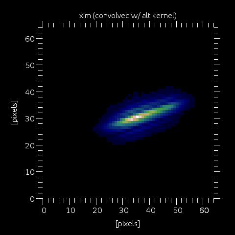
Step 6: We then convolve xim by a kernel which will blur the dotty profile above by a kernel align with the LGS elongation. The LGS profile is now the combination of a number of weighted diracs, convolved by a small kernel of FWHM defined by wfs.gsdepth and typically equal to the separation between the diracs (separation between two points in lgs_prof_alt). I call that an hybrid approach. In yao version < 5.0, the LGS elongation was modelled as a gaussian profile, and I was just convolving a unique spot by a gaussian kernel along the direction of elongation (radially w.r.t. the LLT position). In yao >= 5.0, one could not use the kernel and just choose to have a large number fo points in lgs_prof_amp/alt, but that would take a heavy toll on computing time. Using the hybrid lgs_prof_amp/alt + small elongation kernel gives the best of both world: One can have any arbitrary LGS profile, and still keep limit computing time requirements. Note that there is a utility function, called fit_lgs_profile(), which return the lgs_prof_amp/alt vectors, together with wfs.gsdepth. For most profiles, a fit with 5 to 7 points is sufficient.
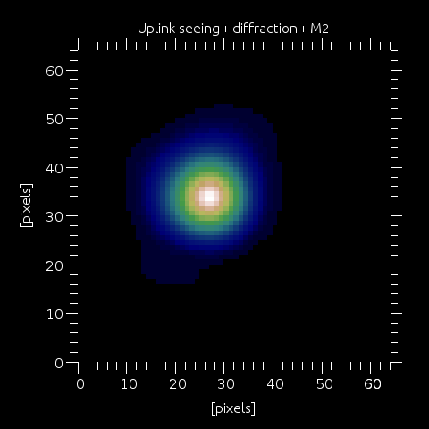
Step 7: From version 5.1, yao includes the option of modelling the effect of the uplink seeing (and laser M2). This is controlled by wfs.LLT_uplink_turb (0|1), with relevant parameters being wfs.LLTr0 (r0 at the LLT and at wfs.lambda wavelength), wfs.LLTdiam and wfs.LLT1overe2diam (the LLT diameter and the laser beam 1/e2 diameter) and wfs.LLTlaserM2 (the laser M2). If wfs.LLT_uplink_turb is set, then all of these effects are computed and an overall kernel is generated (image on left).
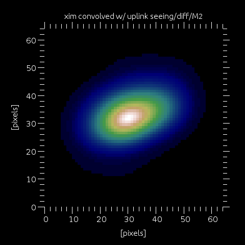
Step 8: xim is convolved with the uplink seeing/M2 kernel. If wfs.LLT_uplink_turb is NOT set, but wfs.kernel is non-zero, then the kernel is a 2D gaussian of FWHM wfs.kernel (arcsec). This was the way yao simulated the LGS extent before version 5.1.
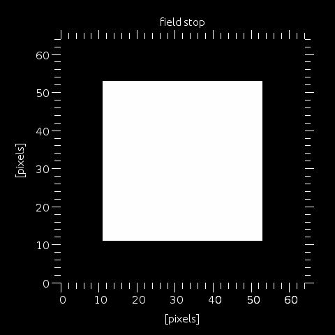
Step 9: This is the field stop, defined by wfs.fstop ("none", "square" or "round") and wfs.fssize (in arcsec).
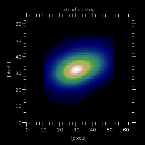
Step 10: xim is multiplied by the field stop.
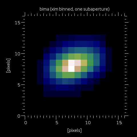
Step 11: xim is binned to the final image desired pixel size. Note that the binning factor has to be a integer number, so that the final pixel size has to be a multiple of the quatum pixel size (see more on that in the main manual).
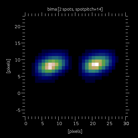
Step 12: All spots (here, an example with 2 of these) are placed in the final SHWFS image, with pitch/separation defined by wfs.spotpitch. Note that now (5.0+) the field of view (extfield), the field stop size and the spot pitch are independently defined, so that one can easily model subaperture interaction, or make sure there's no wrapping possible by using a large enough extfield and keeping the field stop size and spotpitch to the desired value (i.e. a spot can not wrap back, disapearing on the left to appear on the right by property of the FFT), etc...
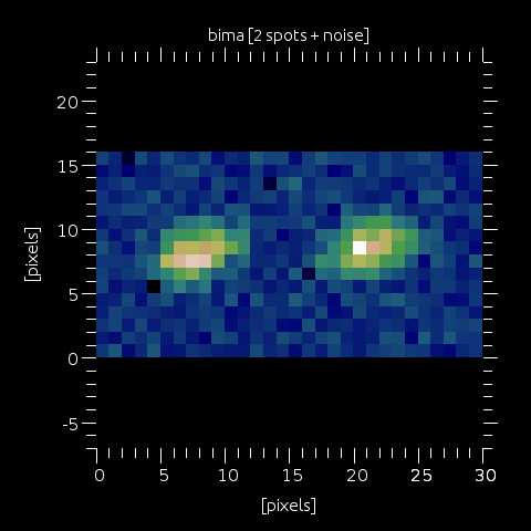
Step 13: Add noise, darkcurrent, take into account effects of bias & flat, etc...
Sometimes pseudo code is easier to understand than words. Here is the pseudo code for the shwfs processes described above:
:
for each subapertures
    for each defocus values (=each point in LGS profile)
        * extract phaselet in front of subaperture
        * fit tiptilt at best
        * remove fitted tiptilt from phaselet
        * embed in larger array (power of two greater than size*2)
        * compute image sim
        * embed sim in xim at coordinate computed from previous tiptilt fit
          (note: accumulate/add to xim content)
    end loop on defocus value
    * convolve xim by elongation kernel (subaperture dependent)
    * convolve xim by uplink/M2 or gaussian kernel (common to all subapertures)
      (note: the last 2 operations are in fact done together)
    * normalize for flux
    * apply field stop
    * bin
    * embed bin image into final SHWFS spot image
end loop on subapertures

