A session at a glance...

A basic yao session

... consist of a few steps:

1. Craft up a parameter file describing the system you want to model, say "mysystem.par"
2. Start yorick/yao
3. aoread,"mysystem.par"
4. aoinit,some keywords...
5. aoloop,some keywords...
6. go

Let us now enter into some details.

The Basics

Is yorick installed ? All set up as per the installation instructions ? Then go to the examples directory of the yao distribution; this might be in different locations depending on how you installed yao. To determine where is it is, run the command find_examples_path() within yao. Type the following at the unix prompt:

poliahu:~ $ yorick -i yao.i
 Copyright (c) 2005.  The Regents of the University of California.
 All rights reserved.  Yorick 2.1.05x ready.  For help type 'help'
 Yao version 4.5.0, Last modified 2009oct23
>

You get the yorick and yao welcome messages and the yorick prompt. Alternatively, you can start a normal yorick session and then include yao at any time by typing:

> #include "yao.i"

You can double check everything is normal by typing:

> info,aoread
func aoread(parfile)

if you get this message, you are in business. If not, fix your yorick installation. Click here to show/hide notes on Yorick.

The first thing to do is to create phase screens (to simulate turbulence). Type

> create_phase_screens,2048,256,prefix="screen"

This will create N (N=long dimension/short dimension, 8 in that case) phase screens of dimension 2048x256 suitable for use by yao. It is advised to choose dimensions that are powers of 2. Depending on your platform and CPU, it may take some time (1mn or so), as this routine is absolutely not optimized. This is a one shot run. You will not need to do that everytime you run yao, as you can, and are encouraged, to use the same phase screens. You may need to run it once more to create larger phase screens if the need arises, but that's about it. The phase screens (screen1.fits to screen8.fits in the example above) will be created in the current working directory. Move them somewhere convenient (I have them in Y_USER/data=.yorick/data in my case). You will need to edit the yao parameter files to reflect the path and names of these phase screens if you put it somewhere different or used a different name (look for "atm.screen" in the parfile).

Next, we will try to run "sh6x6", which is a simple 6x6 Shack-Hartmann example. After you have edited the "sh6x6.par" file (in the examples directory) and modified the path and filename of the newly created phase screens, if needed, type:

> aoread,"sh6x6.par"
Yao, Version 4.5.0, 2009oct23
Checking parameters ...
No field stop defined for wfs 1. Setting to 'square'
wfs(1).fssize has not been set, will be forced to subap FoV
dm(1).coupling set to 0.200000
dm(1).iffile set to sh6x6-if1.fits
dm(2).iffile set to sh6x6-if2.fits
OK
>

What aoread() does is (a) read, or rather include, the parameter file, which will fill the various structures containing the definitions of the WFS, DM, loop, etc... and (b) go through a simple check of the parameters to see if anything is missing or if there are incompatible assigments, in which case it will print out an error message (hopefully understandable). Otherwise, it prints out informational messages or warnings.

Then we need to initialize the system. aoinit() will do that for us. It will initialize all the arrays (pupil, etc), initialize the system pupil, the various WFS, DM, etc. It will then compute the interaction matrix, invert it and finally plot (if requested) a graphical system configuration. The amount of information you get during the aoinit is set by sim.verbose. The default verbose in sh6x6.par is 0, which means you get no feedback at all except for warnings and error messages. Let's set sim.verbose to 1 and run aoinit():

> sim.verbose=1
> aoinit,disp=1,clean=1
Checking parameters ...
OK

> INITIALIZING PHASE SCREENS
Reading phase screen "~/.yorick/data/screen1.fits"
Reading phase screen "~/.yorick/data/screen2.fits"
Reading phase screen "~/.yorick/data/screen3.fits"
Reading phase screen "~/.yorick/data/screen4.fits"

> INITIALIZING SENSOR GEOMETRY
Kernel FWHM for the iMat calibration = 0.364983
Pre-computing Kernels for the SH WFS
 WFS# |       Pixel sizes         | Subap. size | Number of pixels | #photons
      | Desired  Quantum  Actual  | Max  Actual | Desired   Actual | /sub/iter
 1      0.20000  0.03182  0.19093   2.04  1.91    10x10      10x10   70735.5
NGS#1 flux varies between 42795 and 70736 photon/subap/it

> Initializing DM influence functions
  >> Computing Influence functions for mirror # 1

Creating Influence function for actuator #1 2 3 4 5 6 7 8 9 10 11 12
13 14 15 16 17 18 19 20 21 22 23 24 25 26 27 28 29 30 31 32 33 34 35
36 37 38 39 40 41 42 43 44 45 46 47 48 49

  >> Storing influence functions in sh6x6-if1.fits... Done
  >> Computing Influence functions for mirror # 2

  >> Storing influence functions in sh6x6-if2.fits... Done

> DOING INTERACTION MATRIX
  DM #1: # of valid actuators: 45. (I got rid of 4 actuators after iMat)
  >> valid I.F. stored in sh6x6-if1.fits
Computing valid to extrap. matrix for DM#1

> INITIALIZING MODAL GAINS
I did not find simulModeGains.fits or it did not have the right
   number of elements (should be 47), so I have generated
   a modal gain vector with ones in it.


> INTERACTION AND COMMAND MATRICES
 >> Preparing SVD and computing command matrice
Smallests 2 normalized eigenvalues = 0.014315    1.62232e-07
4 modes discarded in the inversion

Summary:
Mirror #1, stackarray, 45 actuators, conjugated @ 0 m
Mirror #2, tiptilt, 2 actuators, conjugated @ 0 m
WFS # 1, hartmann (meth. 2), 32 subap., offaxis (+0.0",+0.0"), noise enabled
D/r0 (500nm) = 42.4; 5000 iterations
> 

At this point you have initialized everything. The aoinit() keyword clean indicates that you want to start from scratch, and ignore any influence function or interaction/command matrix files on your disk. The disp=1 is to get some graphical feedback. You are now ready to run the loop:

> loop.niter = 1000
> aoloop,disp=10
NGS#1 flux varies between 42795 and 70736 photon/subap/it

> Starting loop with 1000 iterations
> go
 Iter#  Inst.Strehl  Long expo.Strehl  Time Left
     1  0.000        0.000             00:00:18.8
    51  0.407        0.393             00:00:15.1
   101  0.412        0.410             00:00:13.7
   [...]
   901  0.647        0.504             00:00:01.4
   951  0.546        0.507             00:00:00.7
Saving results in /home/frigaut/yorick-2.1/share/yao/examples/sh6x6.res (ps,imav.fits)...
time(1-2) =  9.49 ms  (WF sensing)
time(2-3) =  0.03 ms  (Reset and measurement history handling)
time(3-4) =  0.01 ms  (cMat multiplication)
time(4-5) =  1.85 ms  (DM shape computation)
time(5-6) =  1.44 ms  (Target PSFs estimation)
time(6-7) =  1.53 ms  (Displays)
time(7-8) =  0.05 ms  (Circular buffers, end-of-loop printouts)
Finished on 00:26:30
69.040800 iterations/second in average

         lambda   XPos   YPos  FWHM[mas]  Strehl  E50d[mas]  #modes comp.
Star# 1    1.65    0.0    0.0       44.1   0.507      172.0         35.1
Field Avg  1.65                     44.1   0.507      172.0
Field rms                            0.0   0.000        0.0
> 

You have ran 1000 iterations (loop.niter in sh6x6.par is larger so we changed it before starting the loop in the example above to keep your demo time reasonable -note if you want to make it larger than the initial value, you will need to re-run aoinit()). disp=10 in the call means "do your displays every 10 iterations". Depending on your graphic card, displays can be pretty expensive (time), thus it helps to display less frequently.

At any time, while the loop is running, you have access to the yorick prompt. You can type regular commands, but the most useful are:

• stop which will pause the execution of the loop,
• cont which will resume the loop where it paused,
• reset which will reset commands and dm shape,
• restart which will restart from iteration 1.

at the completion of the requested number of iterations, go() will automatically call the function after_loop(), which outputs a number of things as shown above (starting from "Saving results..."): Some statistics on execution time and number of iterations per seconds, and the Strehl, FWHM, etc, on every "target" for which positions were specified in the parameter file. You can call after_loop() by hand at any time also, and you can call it multiple times.

The resulting average images have been saved on disk ("sh6x6-imav.fits"), together with a small postscript file ("sh6x6.ps") that contains some graphics. Strehl, FWHM and 50 percent encircled energy are available as extern variables under the name strehl, fwhm and e50 (the averaged PSFs are also available, together with the history of DM commands, DM errors and WFS measurements if the keyword savecb= has been set):

> strehl
[[0.434317]]

These variables contains the values for all the images (here there is only one, but there can be an arbitrary number of positions and wavelengths at which you want to estimate the performance). This can be useful in script, as detailled below.

Finally, note that you can have access to some documentation on each function by typing help,function_name, e.g:

> help, aoinit
 /* DOCUMENT aoinit(disp=,clean=,forcemat=,svd=,dpi=,keepdmconfig=)
    Second function of the ao serie.
    Initialize everything in preparation for the loop (aoloop).
    Follows a call to aoread, parfile.

    disp         = set to display stuff
    clean        = if set, aoinit will start fresh. *Nothing* is kept from
[...]

> info, aoinit
func aoinit(disp=,clean=,forcemat=,svd=,dpi=,keepdmconfig=)

The Parameter File

Here is an example of a parameter file (parfile). Comments below.

// YAO parameter file
//-------------------------------
sim.name           = "SH6x6 w/ TT mirror and WFS, full diffraction WFS";
sim.pupildiam      = 120;
sim.debug          = 0;
sim.verbose        = 0;

//-------------------------------
atm.dr0at05mic     = 42.44;  // this is r0=0.166 at 550 nm
atm.screen	   = &(Y_USER+"data/screen"+["1","2","3","4"]+".fits");
atm.layerfrac      = &([0.4,0.2,0.3,0.1]);
atm.layerspeed     = &([11.,20,29,35]);
atm.layeralt	   = &([0.,400,6000,9000]);
atm.winddir        = &([0,0,0,0]);

//-------------------------------
nwfs               = 1; // number of WFSs (>1 if e.g. mcao)
wfs                = array(wfss,nwfs);

wfs(1).type	   = "hartmann";
wfs(1).lambda	   = 0.65;
wfs(1).gspos       = [0.,0.];
wfs(1).gsalt       = 0.;
wfs(1).gsmag       = 5.;
wfs(1).shmethod	   = 2;
wfs(1).shnxsub	   = 6;
wfs(1).pixsize     = 0.2;
wfs(1).npixels     = 10;
wfs(1).noise       = 1;
wfs(1).ron         = 3.5;
wfs(1).shthreshold = 0.;
wfs(1).nintegcycles= 1;
wfs(n).svipc       = 2;

//-------------------------------
ndm                = 2;
dm                 = array(dms,ndm);

n  =1;
dm(n).type	   = "stackarray";
dm(n).nxact	   = 7;
dm(n).pitch	   = 20;
dm(n).alt          = 0.;
dm(n).unitpervolt  = 0.01;
dm(n).push4imat    = 100;

n  =2;
dm(n).type	   = "tiptilt";
dm(n).alt          = 0.;
dm(n).unitpervolt  = 0.0005;
dm(n).push4imat    = 400;

//-------------------------------
mat.condition      = &([15.]);

//-------------------------------
tel.diam	   = 7.9;
tel.cobs	   = 0.1125;

//-------------------------------
target.lambda	   = &([1.65]);
target.xposition   = &([0.]);
target.yposition   = &([0]);
target.dispzoom    = &([1.]);

//-------------------------------
gs.zeropoint	   = 1e11;

//-------------------------------
loop.gain	   = 0.6;
loop.framedelay    = 1;
loop.niter	   = 5000;
loop.ittime	   = 2e-3;
loop.startskip     = 10;
loop.skipevery     = 10000;
loop.skipby        = 10000;
loop.modalgainfile = "simulModeGains.fits";

//-------------------------------

The parfile defines entirely your system. It consists of nine subsections in which the yao structures are filled. All of the structure members are listed in the yao structure section, together with a short explanation of each parameters (structure member). How to combine these parameters to get yao to do what you want is explained in the controlling features section below.

Several comments:

• A parfile, and the one above in particular, does not have to include all parameters. Only a few are mandatory for each elements (WFS, DM) and the rest have reasonable defaults.
• The parfile is in fact a yorick include file, and those are yorick statements you see in there. So you can make use of yorick loops, etc (see for example mcao2-bench.par on how the wfs structure is filled).
• Because they can have variable length, and be dynamically re-defined, many structure members are actually pointers (to vectors or arrays). A pointer in yorick is assigned with the symbol & so that &a is the pointer to the quantity a. The notation

  atm.layerfrac = &([0.4,0.2,0.3,0.1]);

  is a shorthand for

  a=[0.4,0.2,0.3,0.1];
  atm.layerfrac = &a;

  If you forget the & sign, it should generate an error.
• There are about 20 parfiles in the example directory (remember? find_examples_path() will tell you where this directory is). Browse through these examples. It is recommended to actually start from one of these, preferably one that is close to the system you want to simulate, and adapt it to your needs, rather than starting from scratch.
• Once you are done, save the parfile and, in the same directory, start yao and go through the sequence of aoread(), aoinit(), aoloop() and go() as shown in section 1.

Controlling Features

Overall Geometry

In yao, you have to define the AO system you want to simulate. It starts by defining an entrance aperture (the system pupil). This is done through 2 parameters: the physical pupil size (e.g. diameter) in real world units, meters. And because yao is a monte-carlo code, that uses arrays to generate phases and PSFs, we will need a pupil array and thus a pupil diameter in pixel.

sim.pupildiam  <- this is the pupil diameter in pixel (unitless)
tel.diam       <- this is the telescope diameter in meters

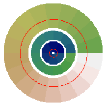
Typical geometry of a system (WFS and DM)

yao also uses arrays to store the deformable mirror influence functions, etc. Generally speaking, there are two types of variable and arrays: the one referring to quantities in the near field (pupil plane or close to it, e.g. altitude layers) and the one referring to quantities in the far field (Shack-Hartmann WFS spots, PSF image, observed object, etc...).

The figure on the right illustrates how you can set up a Shack-Hartmann + Stackarray deformable mirror (allegedly the most common type of AO system to date). I will review all these parameters in sections below, but what I want to emphasize here is the following:

• The pupil is defined on a pixel array
• The WFS has to be defined (at least SHWFS) to span an area commensurate with the pupil (see below). However, it is possible to slightly oversize, downsize or even shift the WFS w.r.t. the pupil, if needed.
• The DM actuator positions and span also has to be defined to span an area commensurate with the pupil and WFS (see below). For a stackarray mirror, for instance, you typically want to have the DM pitch equal to the subaperture size (it doesn't have to be, but it is often the case). As for the WFS, you have the possibility to mismatch WFS and DMs by choosing a different pitch, or shifting the DM to induce misregistration.

Field of view considerations

The size of the pupil is actually quite important. By property of the Fourier transform, the field of view in the far field will be defined by the sampling in the near field, following the relation:

FoV = lambda/ps

Choose the field of view according to your application. But because eventually you will want to run simulations in presence of turbulence, I generally advise to take at least 2 points per r0 (near field), and preferably 3. For r0 = 16 cm, that means a sampling of 8 cm (resp 5.33 cm), and for a 8-m telescope that would translate into 100 points (resp 150) across the pupil (sim.pupildiam = 100). If this is not done, you will likely end up with aliasing in the SHWFS subaperture images (probably less so in the final image if it is estimated in the Near Infrared and the WFS works in the visible). This is bad and will bias your results. You have been warned.

That said, yao 5.0 has introduced a new feature for Shack-Hartmann WFS: extended field of view. When using this feature (control it with wfs.extfield), the individual subaperture imagelets are embedded into larger intermediate images before being binned and embedded into the final SHWFS spot image. This allows extending the field of view of subapertures without the prohibite cost of using a very large number of pixels in your pupil diameter (as outlined above). It is of particular interest for large LGS elongations, e.g. for ELTs. The whole process, describing the steps used to compute the SHWFS final spot image, is somewhat detailled in this page.

Pupil

Historically, yao was developed assuming circular pupils. So in any case, as said above, you will have to define sim.pupildiam and tel.diam. If another pupil shape is desired, it can be defined through a call to a user defined function user_pupil(). Click here to show/hide an example.

func make_square_pupil(void)
{
  extern ipupil, pupil;

  ipupil = array(0.0f,[2,sim._size,sim._size]);
  ipupil(sim._cent-sim.pupildiam/2+1:sim._cent+sim.pupildiam/2,
         sim._cent-sim.pupildiam/2+1:sim._cent+sim.pupildiam/2) = 1.0f;
  pupil = ipupil;
}
user_pupil = make_square_pupil;

Wavefront Sensors

Shack-Hartmann WFS

Set wfs.type="hartmann". The only other mandatory parameters to define are wfs.shnxsub, wfs.npixpersub, wfs.npixels, wfs.pixsize and wfs.lambda. Below I expand on these parameters.

Near Field

The near field parameters that need to be defined are:

• wfs.shnxsub: The number of subapertures in the aperture diameter
• wfs.npixpersub: The number of pixels across one subaperture, in the near field.

For a "normal" system, we want wfs.shnxsub * wfs.npixpersub = sim.pupildiam. But as said above, you can make npixpersub larger or smaller if you want to investigate the effect of subapertures larger or smaller than ideal. Also, by setting wfs.pupoffset [meter], you can investigate the effect of misregistration of the WFS w.r.t the entrance pupil (Show/Hide details).

wfs.pupoffset = [0.03*tel.diam,0.];

Far Field

The far field parameters to define for a SHWFS are:

• wfs.npixels: The number of (CCD) pixel per subaperture in the far field
• wfs.pixsize: The SHWFS (CCD) pixel size, in arcsec.

So that of course, the subaperture field of view will be wfs.npixels * wfs.pixsize. The whole discussion about sampling above of course applies here too, and field of view can not be arbitrary large. The pixel size is also constrained by FFT properties, and yao will round the pixel size you have selected to the nearest possible value (this should be printed out on screen during aoinit if sim.verbose>=1).

Field Stops

Since v4.5.0, yao can handle field stops (before also, but not in the same easy fashion), defined using the parameters wfs.fstop, wfs.fssize and wfs.fsoffset. You have the choice between no field stop (wfs.fstop="none"), or a square or round field stop (wfs.fstop="square" or "round"). If needed, you can use your own defined geometry by setting wfs.fsname to the name of a fits file that contains the image of a field stop (show/hide how). The default is to use a square field stop of size equal to the subaperture field of view (i.e. optimal).

Subaperture Coupling

Shack-Hartmann focal plane features

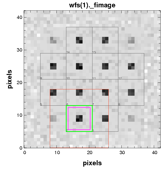
Since v4.5.0, yao correctly includes coupling between neighbor subapertures: In a real system, if there is no field stop, the spot image of a subaperture can wander into a neighbor subaperture and wreak havoc the slope estimation. yao now correctly handle this behavior: all subaperture images are computed, then added to an image that will include all spots. When all spots have been computed, each spot image is extracted and the spot position is estimated from there (center of gravity, soon to come weighted CoG, etc...).

Graphic configuration

When the correct debug setting is selected (sim.debug>=1), aoinit() will display a SHWFS far field graphic configuration diagram as shown on the right (click on it to enlarge). Reported on it are:

• The SHWFS image. This image is accesible to the user in *wfs._fimage, if the need arises. This image includes the spots from all subapertures, including the ones which are not "valid" (because their fractional flux is lower than wfs.fracIllum). The valid subaperture spots are indicated by the thin grey squares.
• For one spot, the diagram plots :
  • the subaperture effective field of view (green square),
  • the total field of view spanned by this subaperture (see discussion on field of view above), in which the spot can wander (red square) and
  • the outline of the field stop (in magenta).

Curvature WFS

Set wfs.type="curvature". The only other mandatory parameters to define are wfs.l, wfs.nsubperring and wfs.lambda:

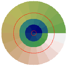
CWFS Subaperture map

• wfs.l is the extra focal distance in an F/60 beam. The first curvature system for astronomy, the UH13, had a WFS input beam of F/60 (on the membrane mirror), and thus use to define extra focal distance in a F/60 beam. I wrote aosimul, the precursor to yao, to model PUEO, the curvature system for the CFHT, which was largely based on UH13. So from then on, to have a common ground, I (and other people) used to quote extra focal distances in a F/60 beam. It is easy to make the conversion to another F ratio, but yao only handles these units.
  Note that the extra-focal image is computed as the Fresnel diffraction of the pupil complex amplitude, using the following algorithm:
  • Fourier Transform the pupil complex amplitude
  • add a quadratic (focus) term with amplitude alpha
  • Fourier transform back
  What you get after that is a defocused pupil image. This has limitations. For instance, it is not possible to compute an image too close to focus, as this would imply alpha = ∞. Of course, this depends of the sampling in the near field, but typically, one can cover reasonable extra focal distances of 5-10cm up (typical systems like PUEO use 15-20cm depending on the seeing, NICI on Gemini uses 40cm).
• wfs.nsubperring: typically, to date, most of the curvature WFS for astronomy were based on a polar design: rings of subapertures. wfs.nsubperring is a pointer to a long vector that contains the number of subaperture per ring: the first element is the number of subapertures in the first ring, the second element the number of subaperture in the second ring, etc.. so that wfs.nsubperring could look like &([6,12,18]) for a system with 3 rings of with 6, 12 and 18 subapertures (the & is because wfs.nsubperring is a pointer). yao automatically computes the inner and outer radius of each ring so that every subaperture receives the same amount of light. The user can modify this behavior by setting wfs.rint and wfs.rout to speficy the inner and outer radius of each ring. (show/hide details).
  

  CWFS, effect of rint and rout

  The subapertures are defined on an array, that is, each pixels of an array of the same size as ipupil belongs to one and only one subaperture. After an aoinit(), you can get a view of the subaperture number map (figure 3) by calling:

  // call again the subap init function:
  subs = make_curv_wfs_subs(ns,sim._size,sim.pupildiam,cobs=tel.cobs);
  // build the one image where pixel value = subaperture number
  submap = (subs*(indgen(wfs(ns)._nsub)(-,-,)))(,,sum);
  // display it:
  fma; pli submap;

  wfs.rint and wfs.rout can modify this behavior and let the user impose his/her own inner and outer radius for each ring. Just set wfs.rint and wfs.rout to the N ring inner radius (in fraction of pupil radius), e.g.

    wfs.rint = &([0.2,0.6,0.9]);
    wfs.rout = &([0.55,0.85,1.5]);
  

  to produce something like on figure 4 (the red line is the pupil outline). This comes handy to take into account dead zones between rings due to glue, etc... We will see later that the same can be done for curvature DM. You can also rotate rings using wfs.angleoffset, which points to a float vector of same dimension as wfs.nsubperring, containing the angle offset per ring. For instance in the figure 4 case, if I wanted to have the external ring rotated 90 degrees CCW so that the green/white subaperture edge is at 12:00 o'clock, I would use wfs.angleoffset = &float([0,0,90.])

Pyramid WFS

Briefly: The Pyramid WFS, in yao, is defined very similarly to the SH WFS. You have to define wfs.shnxsub (# of subapertures in pupil diameter), and the number of pixels in the pupil/phase plane per subaperture, wfs.npixpersub. For instance, if you want to simulate a pyramid WFS with 8x8 "subapertures" (pixels in pupil image), you can use: wfs.shnxsub=8, wfs.npixpersub=8, in which case sim.pupildiam=64. Currently, we can't have sim.pupildiam != wfs.shnxsub * wfs.npixpersub.

Other parameters used by the pyramid WFS only are listed in the structure table below. They are commented and fairly self-explanatory. Note that it is important (and required) to set a field stop when working with pyramid wfs in yao. The way it's implemented, the execution speed depends on the field stop diameter, so don't be surprised. Use a field stop large enough to avoid aliasing and growth of waffle like modes.

Zernike WFS

Set wfs.type="zernike". The only other mandatory parameter is wfs.nzer, which, as its name says, define the number of zernike in the WFS. Note that this include piston, so wfs.nzer=11 would include up to spherical (included). Important note: The Zernike are the Noll Zernike (see Noll 1976), which are not the standard Zernike, but the one used most commonly in AO.

User defined WFS

Set wfs.type="name_of_your_function".

Users can define their own WFS, to be integrated into the yao flow. The API are relatively straighforward:

func user_wfs_func(ipupil,phase,ns,init=)

• ipupil and phase are the pupil and phase (size sim._size),
• ns is the WFS number (as defined in the parfile), and
• init is just a flag set the first time this function is called (in aoinit()) that allow the user function to make some initializations, if needed.

The function should return a measurement vector (show/hide example).

func piston_wfs(pup,phase,ns,init=)
{
  if (init) {
    /* do whatever you need to do and keep possible
       init variable in extern
       here we don't need to init anything. */
  }
  return avg(phase(where(pup)));
}

Photometry and noise

Photometry and noise are only relevant (and implemented) for Shack-Hartmann and Curvature WFS.

All the photometry is controlled with the wfs.gsmag, wfs.skymag and wfs.zeropoint. wfs.zeropoint is defined in photons/second/full_aperture (incident on the telescope aperture, i.e. after crossing the atmosphere). Note that this depends on the telescope diameter (may be it was a bad choice to define it like that, but now it's done). It is simple enough to convert known photometric zero point to yao zeropoint. The number of photons available for WFSing is derived from this zeropoint and the above mentioned magnitude following regular equations (see also wfs.optthroughput).

yao doesn't have a concept of ADU. Or rather, I am assuming one electron/ADU across the board. So the signal in in electrons, and the noise is also in electrons.

Deformable Mirrors

The deformable mirrors are entirely and solely defined through their influence functions (shape and location). During the aoinit() phase, yao calls DM influence function definition functions, for each DM in the parameter file. Once computed, the influence functions are stored in the dm structure (*dm._def) and saved on disk for future runs (name-if#.fits files). Note that if you have a set of commands, you can get the DM surface by calling

surf = compute_dm_shape(nm,command_ptr);

where command_ptr is a pointer to a float vector containing the DM commands (e.g. command_ptr = &(float(indgen(dm._nact)))).

Stackarray (PZT,SAM,Piezo) DM

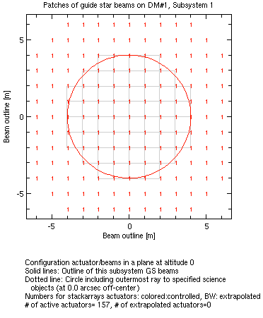
Set dm.type="stackarray". The only other mandatory parameters for stackarrays are dm.pitch and dm.nxact.

Dimensioning

dm.nxact sets the number of actuators in the diameter of the DM (along the X or Y axis). This includes extrapolated/slaved actuators/guard rings.

dm.pitch sets the pitch (i.e. interactuator distance) in near field pixels.

Note that you have to dimension the stackarray DM according to your base system definition (sim.pupildiam). If you set sim.pupildiam=60 and dm.nxact=7 and you do not desire an extra ring of actuator, then you should set dm.pitch=10 to span the entire pupil diameter (7 actuators, 6 spaces between actuators...).

Influence functions

This was the first type of DM implemented in yao. With time, we have implemented several type of influence functions. By default, it uses a functional form which was first derived by J.-P. Gaffard of then CGE (now CILAS) to fit ZIGO measurements of CGE DM's real influence functions. It is possible to use newer (but not necessarily better) forms by setting dm.irexp:

dm.irexp	functional form
0	Old, adhoc functional form fitted on actual ZIGO data
1	exp(-(d/irfact)^1.5)
2	sinc*gaussian

irfact is set through dm.irfact.

Actuator Coupling

You can set the inter-actuator coupling with dm.coupling. dm.coupling=0.3 means 30% coupling between an actuator and its nearest neighbor. Typical value are 0.1-0.4. The almost universal consensus nowadays is to use coupling values of about 0.3.

Saving RAM & Disk with dm.elt

Stackarray mirrors have very local influence functions. Therefore, for large number of actuators, most of the surface of the DM is zero. It is thus a big waste of RAM and disk (these influence functions take a lot of space). Enabling dm.elt will save most of this space back: only a small subsection of the whole DM surface is kept, surrounding the actuator. The coordinates of this subimage is kept, and used later by comp_dm_shape() to compute the correct DM shape. The call to comp_dm_shape() is transparent. Depending on the value of dm.elt for the current DM, comp_dm_shape() will call the relevant C routine. In fact, there is no compromise in setting dm.elt, but its benefit really only show up for large stackarray DM (dm.nxact≥10).

Extrapolated/Slaved actuators

The idea in yao is to define all of your stackarray mirror in your parameter file, then run aoinit() and calibrate the iMat, then select which actuators are controlled and which are extrapolated based on the WFS sensitivity to it. Use dm.thresholdresp to select this threshold. This is a fractional number, so 1 would filter all actuators and 0 would retain them all. 0.5 would retain all actuator which measurement max response is larger than the max response of all actuators. Note that if you set dm.thresholdresp to a negative value, aoinit() will enter an interactive mode into which you can test various values of dm.thresholdresp (Show/Hide example).

In this example, I have a SHWFS with 8x8 subapertures and a stackarray DM with 13x13 actuators. The relevant parts of the parfile are as follow:

sim.pupildiam       = 256;

wfs                 = array(wfss,1);
wfs(1).type         = "hartmann";
wfs(1).shnxsub      = 8;
wfs(1).npixpersub   = 32;
wfs(1).lambda       = 0.65;
wfs(1).pixsize      = 0.25;
wfs(1).npixels      = 8;

dm                  = array(dms,1);
dm(1).type          = "stackarray";
dm(1).nxact         = 13;
dm(1).pitch         = 32;
dm(1).alt           = 0.;
dm(1).thresholdresp = -0.1;

After doing the iMat calibration in aoinit(), and if dm.thresholdresp<0, you will be presented with the figure shown above on the left. Notice that all actuators are red, which means they are currently all valid. In the yorick console, yao will write the current number of valid actuators. Answer "y" and enter a new threshold (here I entered 0.5). The plot updates (see figure above on the right) and now shows valid actuator (still in red) and extrapolated actuators (now in foreground color -here black-). Once you are satisfied, answer "n" to "Again?" and yao will proceed.

DM #1: # of valid actuators: 157 Again ? y
Threshold (old = -0.100000) : 0.5
type return to continue...
DM #1: # of valid actuators: 69 Again ? n
  DM #1: # of valid actuators: 69. (I got rid of 88 actuators after iMat)
  >> valid I.F. stored in test-if1.fits

Once extrapolated actuators are selected, yao stores the valid influence functions and the extrapolated ones in 2 different files (e.g. test-if1.fits and test-if1-ext.fits). Influence functions are not recomputed in further calls to aoinit() unless the clean keyword is set (in which case aoinit() restart from scratch and recompute everything).

Bimorph (curvature) DM

Set dm.type="bimorph". The other mandatory parameter is dm.nelperring.

dm.nelperring: This is similar to wfs.nsubperring (see here) and defines the number of electrodes per ring.

Now, most curvature mirror are a bit different from this simple design provided by defining dm.nelperring, in which there is no gap between rings. Many curvature DMs have for instance a large gap between the outer ring of electrodes (the one that create mostly boundary conditions) and the next inner electrode ring. To create more realistic DM electrode pattern, use angleoffset, rint, rout, supportRadius and supportOffset.

The general idea follows what has been exposed in the curvature WFS area above. With rint and rout, one can define the inner and outer radius of each ring of electrodes, expressed in fraction of the pupil radius. With angleoffset, one can define a global rotation per ring, and with the support* parameters, one can define the physical properties of the 3 DM support points.

That brings us to the next subject: how curvature DMs are modelled. Right now, what we do is solve the Poisson equation, imposing a given curvature over a given electrode and integrating twice to get the DM surface. Then, we impose that the three points defined as the support location go through the z=0 plane. It's that simple. It means that we do not currently support fancier support method like continuous support (e.g. by a rubber ring), 6 points support, etc..

Modal (Zernike, Disk Harmonic, Karhuenen-Loeve) DM

Set dm.type="zernike","diskharmonic" or "kl". Other mandatory keywords are dm.nzer (for zernike), dm.max_order for disk harmonic or dm.nkl (for KL), which specify the number of modes. Note that nzer (Zernike) & max_order (disk harmonic) will start and include piston, while nkl (KL) will not (there is formally no piston mode in the KL basis).

Segmented DM

Set dm.type="segmented". The other mandatory keywords is dm.nxseg.

dm.nxseg is the number of segment in the long diameter (X axis).

dm.fradius stands for "filter radius". Segments are created over a wider area than the nxseg defined above. Only segments which distance to the (0,0) pupil coordinates is ≤ fradius will be kept. default dm.pitch*dm.nxseg/2.

User defined DM

Set dm.type="name_of_your_function" (as a string).

The API for the user provided DM function are as follow:

func make_my_dm(nm,disp=)

func make_my_dm(nm)
{
  extern dm;   // dm is extern (global)
  dim = dm(nm)._n2-dm(nm)._n1+1; // <- important
  def = array(float,[3,dim,dim,n_actuator]);
  for (i=1;i<=n_actuator;i++) def(,,i) = some_form; // <- fill it to your taste
  dm(nm)._def = &def;  // <- store influence functions
  dm(nm)._nact = n_actuator;  // <- important, number of actuators
}

Explanation: In this user supplied function, you have to define the influence functions (*dm._def) and, importantly, the number of actuators (dm._nact). Prior to the call to this function, aoinit() has defined dm._n1 and dm._n2, which are the indices at which these influence function will go in the big sim._size x sim._size array used for FFT, etc. The influence functions are reduced in size to save RAM, as they can potentially take a lot of memory space. Normally, dm._n1 and dm._n2 are defined to include the pupil pixel diameter (sim.pupildiam) plus 4 pixels padding on each side if the DM altitude is zero (in the pupil), and are defined to span the entire sim._size array if the DM altitude is above ground (as there is no simple way to know where to stop exactly as this depends on the WFS and target locations). Note that dm is defined in extern as you are modifying its value.

Tip-Tilt Mirror

Set dm.type="tiptilt".

This creates a regular tip-tilt mirror. The units in the command vector are arcsecs.

Anisoplanatism "DM"

Set dm.type="aniso".

This has been implemented because of the need in MCAO to control plate scale modes (also called anisoplanatism modes or quadratic modes). You will need to set dm.alt to the altitude of an existing DM of a regular type (e.g. stackarray) that will be responsible for the creation of the anisoplanatism modes (see mcao2-bench.par for an example of aniso DM).

Hysteresis and misregistration/offset

Hysteresis

Hysteresis is implemented at the top level so that it works for any kind of DM (during the AO loop only). The parameter dm.hysteresis is fairly self explanatory: dm.hysteresis=0.1 means 10% hysteresis.

Misregistration

dm.misreg allow to induce DM misregistration (on the fly). dm.misreg is expressed in pixels, so you will have to do a small conversion to get it in other units, but this way, it works for any kind of DM. Note that dm.misreg can be fractional (fraction of a pixel). Because the size of the array containing the DM influence function is limited to save memory space, the misregistration using this parameter can only be of a few pixels (up to 4 I believe for a ground-conjugated DM). If you wish to induce more registration, use the parameter dm.pupoffset (see below).

Offsets

Yao v4.5.0 introduced a new kind of influence function offset parameter: dm.pupoffset. dm.pupoffset is entered in meters (a 2 elements vector which contains the x and the y offsets). Those are transversal offset of the influence functions in the near field. This functionality is implemented in the compute_dm_shape() function, so it is general and works for all types of DM. dm.pupoffset is intended for large offsets, and the influence functions are shifted by an integer number of pixels (the requested offset in meter, rounded to the nearest pixel, see sim.pupildiam and tel.diam). If you want finer control over the DM position, use dm.misreg (see above). dm.pupoffset is similar to wfs.pupoffset (see WFS section), but for the DMs.

Building a Reconstructor

The default reconstructor which was initially the only option in YAO is the truncated singular value decomposition (SVD). This is a least-square solution where invisible or poorly sensed modes are totally discarded. A faster and better performing reconstructor (especially for large AO systems) is the minimum mean-square error (MMSE) reconstructor. This MMSE reconstructor can be either built using full matrices or sparse matrices techniques, which offers a significant speed boost.

Method selection

There are three options for wavefront reconstruction, and these are set using the mat.method parameter.

Truncated singular value decomposition (default)

mat.method = "svd"
mat.condition = &([desired conditioning])

Minimum Mean Square Error Reconstructor

This method computes the reconstructor as

where H is the interaction matrix (poke matrix), a is a regularization parameter and C is a regularization matrix. The regularization matrix (see dm.regtype or dm.regmatrix) can be user specified or computed by YAO. If it is computed, it will use an identity matrix by default, or a matrix created by convolving a laplacian operator by itself. This matrix has similar statistics to the inverse covariance matrix for Kolmogorov turbulence and penalizes local waffle in the DM.

The relevant parameters for the MMSE inversion process are

    mat.method = "mmse";
    dm.regparam = 0.01; // higher for larger systems
    dm.regtype = "laplacian"; // "laplacian" or "identity"
    dm.regmatrix = &([]); // you can specify your own regularization matrix

Minimum Mean Square Error Sparse Reconstructor

A sparse matrix implementation of the above is also available. This is ideal for very large systems with thousands of actuators, as it reduces memory requirements and increases computational speed. Do not use the sparse method when the interaction matrices are not actually sparse (e.g., when using a Zernike DM).

  mat.method = "mmse-sparse";
  mat.sparse_MR = 1e4; // a number larger than the total number of rows
  mat.sparse_MR = 1e5; // a number larger than the number of elements
  dm.regparam = 0.01; // higher for larger systems
  dm.regtype = "laplacian"; // "laplacian" or "identity"
  dm.regmatrix = &([]); // you can specify your own regularization matrix

If you set the values of mat.sparse_MN and mat.sparse_MR too low, the system could crash. Too high and you could run out of memory.

Code Your Own Reconstructor

It is possible to code your own reconstructor and make YAO use it. You need to overwrite the reconstructor matrix cMat as the matrix that you compute. You can also save the reconstructor so that it is not overwritten whenever aoinit is run.

    cMat = myNewReconstructor;
    yao_fitswrite,YAO_SAVEPATH+mat.file,[iMat,transpose(cMat)];

Your reconstructor will, however, be overwritten if you do aoinit,clean=1 or aoinit,svd=1

Loop parameters

  loop.method     = "closed-loop";
  loop.framedelay = 1;
  loop.gain       = 0.6;
  loop.leak       = 0.001; 

The gain is typically a value around 0.5, and the leak is a small value needed to prevent the build-up of poorly sensed modes on the DM. The framedelay is the compute time rounded to the nearest number of frames, typically 1. There is already a one cycle delay inherent in the zero-order hold of the WFS and the DM stare, and this does not need to be added.

For tomographic reconstructors, you can use pseudo open-loop control: loop.method = "pseudo open-loop". If you have an AO system where the WFSs see the uncorrected wavefront, you can run the simulation in open-loop:

    loop.method     = "open-loop";
    loop.framedelay = 1;
    loop.gain       = 1;
    loop.leak       = 1.; 

In open-loop, it is essential to set the loop gain to 1 and the leak to 1.

It is also possible to create high-order control laws and to control each DM with a separate controller. This is especially useful to separate the tip-tilt and DM control. For example, to implement the control law on dm(1):

dm(1).ctrlnum = &([0.5,0.12,-0.05]);
dm(1).ctrlden = &([1,-0.64,-0.36]);

Running yao using parallel processes

More work on yao parallel:

• I have merged some of the -useful- parallel features implemented in our Gemini local yao_mcao to the yao trunk. Namely,
  • The DM/WFS parallelization (meaning, taking advantage of the fact that real systems have at least one frame delay (remember that even if the command is applied immediately after the measurements are received, there is still one frame delay due to the zero order hold). The one frame delay means the WFSing at iteration N is not needed to compute the command at iteration N, thus can be computed in parallel.
  • The PSF calculations, which is a no brainer.
• I have implemented the parallelization of individual SHWFS. Meaning, an individual SHWFS can now run in parallel on an arbitrary number of "threads" (in fact, forks). This works only for Shack-Hartmann WFS. The good thing is that this is implemented fairly deep into the code, so any call to sh_wfs() will benefit from this, which means the iMat acquisition is accelerated too.

Depending on your system, i.e. WFS order, number of WFSs/DMs, whether you use dm.elt or not, sparse reconstructor or not, and more importantly, on the machine you run yao on, using the parallel features can make you gain anywhere between 20% and 200% in execution speed. If you want to use it, you will most probably have to experiment a bit to see what option should be set. Guidelines are given in the manual. The bottom line is that you should not use more forks (processes) than you have CPUs, otherwise swapping processes in/out of L2 cache introduce an overhead which cancels the paralleization advantage. With my core2duo laptop, I can typically gain 30 to 50%. With an 8 cores Xeon-based machine we have at work, I gain typically close to a factor of 2 (can be more or less). This does not seem particularly impressive, but one has to consider that a yao loop is made of many different individual operations: WFS, cMat product to retrieve the error, DM shape computation from the DM commands and the influence functions, PSF calculation, etc... So a gain in one of this items is only going to benefit the whole thing marginally. As far as the individual WFS parallelization is concerned, here are some hard numbers:

8 Core Xeon (2 boards) @ 3.33GHz, running RHEL 5, 32 bits. yorick/yao built with -O2.
16x16 SHWFS system, physical model, no noise. All times (avg & median) in milliseconds for one frame.

sh16x16_svipc:        1 threads, sh_wfs() avg=2.86, median=2.90
sh16x16_svipc:        2 threads, sh_wfs() avg=1.87, median=1.89
sh16x16_svipc:        4 threads, sh_wfs() avg=1.37, median=1.37
sh16x16_svipc:        8 threads, sh_wfs() avg=1.14, median=1.15
sh16x16_svipc:       16 threads, sh_wfs() avg=2.33, median=2.30

You can see that the speed increases up to 8 forks (max gain = 2.5x). Adding more forks makes the thing slower. The gain does not reach larger value just because (1) there are overheads associated to the use of shared memory/semaphores and (2) there is also a global overhead in the sh_wfs() function. What's parallelize is the core of sh_wfs() (FFTs, noise application and slopes calculations from spots), but any overhead within the sh_wfs() function itself, before calling the FFT/slopes calculation routine is not going to gain from the parallelization.

The gain brought by the other, more general parallel features (DM/WFS & PSFs) is nicely illustrated by the following examples. This was run on the same machine (8 cores Xeon), with curvature.par (36 subapertures curvature system ran on a 120 pixels pupil). Look at the following results (I have omitted the timing results for items that are not of concerned here and were negligible):

sim.svipc=0 (no parallelization)
time(1-2) =  9.89 ms  (WF sensing)
time(3-4) =  0.01 ms  (cMat multiplication)
time(4-5) =  1.04 ms  (DM shape computation)
time(5-6) =  5.84 ms  (Target PSFs estimation)
59.18 iterations/second in average


sim.svipc=1 (WFS/DM parallelized)
time(1-2) =  4.11 ms  (WF sensing)
time(3-4) =  0.01 ms  (cMat multiplication)
time(4-5) =  0.94 ms  (DM shape computation)
time(5-6) =  5.78 ms  (Target PSFs estimation)
91.43 iterations/second in average

sim.svipc=2 (PSFs parallelized)
time(1-2) = 10.69 ms  (WF sensing)
time(3-4) =  0.01 ms  (cMat multiplication)
time(4-5) =  1.05 ms  (DM shape computation)
time(5-6) =  1.23 ms  (Target PSFs estimation)
76.41 iterations/second in average

That's a typical example. The "no parallel" case is dominated by WFSing (10ms) and PSF (6ms) calculations. When parallelizing the WFS (sim.svipc=1), the WFSing time goes down to 4ms. Indeed, now 6ms of it can be done in parallel with other tasks: here, the PSF calculation that takes 6ms. With sim.svipc=2 (only the PSF are parallelized), the PSF calculation time goes to basically to 0 while the WFSing stays at 10ms. It all makes sense. I haven't put the sim.svipc=3 results as they are a little more difficult to understand and would just introduce confusion.

The individual WFS parallel feature is controlled by the parameter wfs.svipc. The "global" DMs/WFSs abd PSF parallelization is controlled by sim.svipc (bit 0 controls DM/WFS and bit 1 controls PSFs, thus sim.svipc=3 means both are turned on).

Of course, if you want to use yao parallel facilities, you will need to install the yorick-svipc plugin, through most of the normal channels. It runs on Linux (extensively tested) and OsX (somewhat tested).

Parallel implementation gotcha & bugs

It is difficult to code for parallel deployment. Especially for something like yao which offers a lot of various configuration option to the users. I have tested the parallel implementation quite a lot, but I am sure I have left some corners unexplorered/untested. So you might hit some unexpected features. Let me know if you do notice something weird. In the meantime, here is a list of things to watch out for when using the parallel (svipc) thingy (the first three items should not happen. I haven't seen it for a long time. But I originally saw it hence I give you these tricks in the unlikely event it happens) :

• You can safely turn the sim.svipc features on and off within the same session. If you want to use it though, you need to declare it before the aoinit (so re-run aoinit to enable it). You can disable / re-enable at any time after the first init (init is done within aoinit and forks are done within aoloop).
• Be a little more careful with the wfs.svipc. If you wish to change the number of threads within a yao session, you will need to run quit_wfs_forks() to kill (quit) the wfs forks to be able to re-fork WFS processes with the correct parameters. So, for instance, you could do the following:

  > aoread,"some par file"; wfs.svipc=2; aoinit; aoloop; go;
  [...you get your results]
  > quit_wfs_forks
  > wfs.svipc=4; aoloop; go;
  

  This *should* work. As you get acquainted with the parallel extension, I suggest you keep a terminal open on the side, monitoring the yorick processes (htop or gnome-system-monitor does fine on linux). If it doesn't work, or you get lost, just restart the yorick session.
• If you ever end up with semaphores locked, you can easily Ctrl-C your way out of it. But this may left the shared memory / semaphore mechanism in a weird state. Re-run the yao session (including the svip settings) and quit() yorick. This should cleanup the svipc settings. If push comes to shove, you can list your shared memory segments and semaphores with ipcs and manually kill the culprits with ipcrm -M segment for shared memory or ipcrm -S segment for semaphores. The one yao uses generally start at 0x0badcafe (and up) for the shm and 0xdeadbeef (and up) for semaphores. On modern linux systems, this can not harm your machine or the state of your OS. You should never have to reboot as a consequence of using shm/semaphores.
• Before running long simulations, I advise you to check the graphics to make sure everything runs fine. I have seen instances where the forks get desynchonized from the main process, resulting in partial images or noise badly applied.
• Right now the dark feature I believe is broken. Be aware of it and don't use it.

Other Features

More to come (a note to myself).

• disjoint pupils
• loop parameters: framedelay, control law
• Normalization of various parameters and arrays
• Variables (aoinit or not aoinit?)
• Vibrations parametrization

Yao Structures

atm(1).layerfrac = &([0.5,0.2,0.3]);

Scripting and Hacking Yao

Scripting

Thanks to yorick and the structure of yao, scripting is relatively easy. The principle is as follow:

• read the parfile
• init yao (aoinit)
• Loop on parameters you want to loop on:
• set parameters
• if needed, redo the aoinit (some parameters will need that)
• go through the loop N iterations
• store the results
• Plot/save results

Here is a simple example you can find in the examples directory (yao_loop_example.i):

require,"yao.i";

// check if generic phase screens exist, if not, create them:
write,"CREATING PHASE SCREENS";
if (!open(Y_USER+"data/screen1.fits","r",1)) {
  create_phase_screens,1024,256,prefix=YUSER+"data/screen";
 }

// the "wait" is needed here:
window,33,wait=1;

// read out parfile
aoread,"test.par";
atm.dr0at05mic = 35; // be more gentle

// Define vector on which we want to loop and final strehl array.
// We want to estimate performance for 3 values of the guide star
// magnitude and 4 values of the loop gain (for instance)
gsmagv = [6,9,12];           // guide star mag vector
gainv  = [0.01,0.1,0.5,1.0]; // gain vector
// strehl array to store results:
strehlarray = array(0.,[2,numberof(gsmagv),numberof(gainv)]);

// loop on gsmag and gain
for (ii=1;ii<=numberof(gsmagv);ii++) {
  for (jj=1;jj<=numberof(gainv);jj++) {
    wfs(1).gsmag=gsmagv(ii);
    loop.gain=gainv(jj);
    // it's safer, but not always necessary, to call again
    // aoinit (here for gsmag). some parameters do not need it.
    aoinit,disp=1;
    // Setup loop:
    aoloop,disp=1;
    // go: do all loop.niter
    go, all=1;
    // after_loop() is now called automatically at last iter of go()
    strehlarray(ii,jj) = strehllp(0); // fill in result array
    // and display results as we go:
    window,33;
    fma;
    for (ll=1;ll<=ii;ll++) {
      plg,strehlarray(ll,),gainv,color=-ll-4;
      plp,strehlarray(ll,),gainv,color=-ll-4,symbol=4,size=0.6;
      ylims=limits()(3:4); ymax=ylims(2); yspace=(ylims(2)-ylims(1))/15.;
      plt,swrite(format="gsmag=%d",gsmagv(ll)),0.011,ymax-yspace*(ll-1), \
        justify="LT",tosys=1,color=-ll-4;
    }
    logxy,1,0;
    xytitles,"Loop Gain",swrite(format="Strehl @ %.2fmicrons",(*target.lambda)(0));
    window,0;
  }
}

You can do all kind of scripting like this to find for instance the optimal working point for a system in given conditions (above, what is the best gain for a given GS magnitude). We could also have added a loop on wfs.ittime in the example above. One has however to be careful: Probing multi-dimensional spaces can quickly be overwhelming in execution time. Generally, I consider that 10000 iterations are needed to give a statistically significant answer. So for instance, in the example above. that would mean 4x3x10000=120000 iterations total. At 90 iterations/seconds, this means 1300 seconds (about 20mn). Adding 4 points for wfs.ittime would lead to 480000 iterations, or 1 hour and 20mn. This can quickly become prohibitive.

Hacking Yao

At one point or another, if you are serious about simulating your system, it is likely that you will need this or that feature, or modification to the existing yao code.

Go ahead and dive. Feel free to modify yao. It's open source after all. The goal of this too-short section is to give you some head start for doing just that: hacking yao.

So, various points, in no particular order:

• The functions are kind of gathered by themes. The main file is yao.i, and includes the base functions aoread(), aoinit(), aoloop(), go(), after_loop() and more. Other important include files are:
  • yao_wfs.i: All functions related to WFS and their initialization.
  • yao_dm.i: All functions related to DM and their initialization.
  • turbulence.i: Functions to generate turbulent phase screens. Some more turbulence functions are in yao.i
  • yao_structures.i: Definitions of yao structures.
  • aoutil.i and yao_util.i: check_parameters, and in general utility functions that didn't fit anywhere else.
  • yao_fast.i and yao_utils.i: Interface functions to the C routines. Mostly declaration of prototypes as per yorick plug_in APIs.
  • yaokl.i: KL creation functions.
  • yao_fast.c: C code for the SHWFS and CWFS, plus some Poisson and Gaussian noise fast functions.
• Many variables are defined in extern. This means they are available at any level. Here is a subset of them:
  • All the yao structures: wfs, dm, atm, sim, mat, tel, target, gs, loop. There are sufficient examples in the code of how to address them. These will contain most of the information you may want.
  • Variables that may be useful to catch and store/analyze when the loop is finished are (loop in go() and after_loop() for more details):
    • imav(sim._size,sim._size,#_target,#_lambda): the averaged images for each target and at each requested wavelength.
    • strehl(#_target,#_lambda) contains the long exposure image Strehl ratio for each target and each requested wavelength.
    • fwhm(#_target,#_lambda) contains the long exposure image FWHM for each target and each requested wavelength [mas].
    • e50(#_target,#_lambda) contains the long exposure image 50% encircled energy diameter for each target and each requested wavelength [mas].
    • cbmes, cbcom, cberr are the "circular buffers" that contain all WFS measurements, DM commands and DM errors (updates to DMs at each iterations). Only saved if keyword savecb is set in call to aoloop().
  • iMat, cMat: Interaction and control matrices. One axis is the WFS axis. The WFS measurements are put in sequence: all X, then all Y for WFS#1, then all X, then all Y for WFS#2, etc... The other axis is the DM axis. Here also, all valid actuators for DM#1, then DM#2, etc...
  • modToAct, mesToMod, eigenvalues: The U, transpose of V and eigenvalues of the SVD inversion. Over the unmasked eigenvalues, cMat is computed as follow:

    cmat = ( modToAct(,+) * mev(+,) )(,+) * mesToMod(+,);

Conclusion

There is a lot of things missing in this documentation. I will try to complement it as time allows. I hope however that this will help you getting the best out of yao and avoiding frustration. Yao is a fairly complete AO simulation tool. It is flexible and fast. Flexibility means I can not exert too much control over the user input parameters. If I were to do that, I would necessarily impose a straitjacket over your creativity, and we want to avoid this at all cost. So, yes, there is a steep learning curve, but at the end, you should be able to wrestle yao into submission! I have only one more advice to give: check your results. And recheck them. And make sure it makes physical sense.